To appropriately model the sort of data we generally have in reality, simulations of diversification as observed in the fossil record must consider some model of incomplete sampling. In continuous time, the simplest model treats sampling events as a Poisson process, just as the simplest models of speciation and extinction treat those events as Poisson processes. Under this model, the waiting times between events are exponentially distributed with some instantaneous per-lineage-time-unit rate parameter, generally called r (Foote, 1997).
(Tangent on terminology: r matches alright with the general paleobiological usage of p and q for speciation/origination and extinction rates, but not so much for the biological usage which uses lambda and mu for those same rates. Stadler (2010), however, defined sampling rate as a variable (independently possibly, given no references to the paleontological literature) and used psi. For me, though, it'll always be lower-case r.)
Here's an old figure (I need to heavily revise it) from my in-the-works paper on time-scaling methods which illustrates sampling in the fossil record:

As we can see in this simple model, incomplete sampling slices the early and later parts of a taxon's history off, if that taxon is sampled at all. In continuous-time, a majority of taxa will probably have zero-length observed durations ('one-timers'; Foote, 1997). In general, longer-lived taxa will be more likely to get sampled at all and to have positive-length durations, so the probability of sampling any given taxon is not the same.
There are a number of additional complications in how taxa are sampled in the fossil record which make this Poisson model of sampling in continuous time unrealistic. Generally, the ability to temporally resolve the 'date' that any particular taxon is sampled is not so great, and can have considerable error bars. This is generally done with relative dating, using 'biozones', where time is defined based on the appearance of zonal taxa (graptolites happen to be great for this purpose). In some cases, these can be well resolved temporally by correlation with absolute dating (Sadler et al., 2009), for example, Sadler et al. presented global graptolite zones a few hundred thousand years long and for which the start and end dates can be resolved within a few thousand years. However, biozones tend to not extend to the global level and even then the appearance of taxa tends to not by synchronous globally (Sadler, 2011; Loydell, 2012). Some taxa are better than others for defining short biozones. If your Ordovician rocks only have corals, for example, it might be very difficult to correlate those globally with precision, unless other information is available.
Geologists have constructed hierarchical time-scales with eras, periods and stages, all rigorously defined (or proposed to be) based on particular 'type sections', just as Linnean taxa must be based on type specimens. Although we now have global-level systems for much the Phanerozoic (the last ~500 Ma), with the starts and ends of intervals attached to the boundaries between bio-zones, many finds from previous decades are still only reported in terms of more regional systems of intervals, which can be very difficult to correlate to the global system. Thus, in general, our finds are really known from more discretely known intervals, and the order of events within a given interval may be very difficult to resolve. (e.g. A find of Normalograptus normalis within the N. extraordinarius biozone could come from anywhere within the N. extraordinarius biozone.)
In general, a way to deal with these additional complexities of how the nature of correlation and time-scaling of the rock record itself works is to impose a system of discrete intervals on a set of continuous-time sampling events. I think this makes the most sense, as we generally simulate branching processes as the result of instantaneous rates, we should speak of sampling in terms of an instantaneous rate. Some previous studies placed lineages, generated in continuous time, into a discrete time framework and then sample them within those intervals under some per-interval sampling probability. However, the relationship between the instantaneous sampling rate (r) and the per-interval sampling probability (R; Foote and Raup, 1996) is not exactly simple, although it can be loosely approximated (see the function sRate2sProb in paleotree). The per-interval probability assumes taxa span the entire interval, which may not be true as average interval length increases relative to average taxon duration. Also, the discrete time intervals are imposed secondarily by us, the geologists, and so it just makes more sense to me that we should simulate sampling on lineages in continuous time first.
Simulating sampling originally in continuous time actually allows for very quick simulations of sampling. simFossilTaxa makes use of the Poisson process nature of the processes it simulates to only consider the waiting times between events. Its sister function, sampleRanges, does the same thing by default, pulling the waiting times for sampling events from an exponential distribution. It is then very simple to apply binTimeData to the output from sampleRanges, which produces (by default) ranges placed into intervals of equal length, but (as of version 1.3) allows for user-input ranges as an alternative. A future modification may allows for intervals to be defined based on the origin/extinction of taxa, which would be more realistic as the real discrete intervals of the geologic record are often based on such biostratigraphic events (for example, periods were often defined with mass extinctions placed at their boundary, as this created a considerable amount of faunal turnover that allowed for biostratigraphic dissection).
For example, we can simulate sampling on example dataset from the R help file for sampleRanges, with the sampling rate set to 0.5 per Ltu (lineage*time-units). The flat line at top is the (unvarying) sampling rate over time and below it is a diversity curve produced from one simulation of sampling.

For example, we might think that as we get closer to the present, more of the rock record is available and preservation is better so we are more likely to sample taxa. A very simple model of this would be a linear increase in sampling rate over time.
We can simulate this by changing the parameter rTimeRatio, which is basically the increase over time from the start of a clade's origin to its end. The input sampling rate becomes the mean sampling for the dataset in this case (the sampling rate observed at a clade's midpoint. For example, here is a plot of sampling rate for a clade varying over time when rTimeRation=5, along with the observed diversity curve produced by simulating sampling under that model. This plot can be easily reproduced with the examples code in the sampleRanges help page in paleotree 1.3, by the way! You can go run it yourself!

Another model is the 'hat'. Various studies in the last half-decade have suggested that taxa tend to be most abundant and geographically wide-spread in the middle of their geologic duration: the rise and fall of species and genera . Also remarkably, this rise and fall looks like a remarkably normal-looking symmetrical curve. (Lee Hsiang Liow tends to refer to this as the "hat" in her work.) This would lead one to expect that perhaps the rise and fall of taxa might also influence sampling, such that the probability of sampling is highest in the middle of a taxon's temporal range.
sampleRanges can handle this by changing the alpha and beta parameters: when they are set several times higher to 1 and are equal, you get a bell-curve-looking symmetrical distribution. Here, with alpha=beta=4, we get the following, with taxon range represented by a single symmetrical 'hat' of sampling rate increase and decreasing over its range. Again, the sampling rate input (0.5) becomes the 'mean sampling rate' for the dataset.

(A stray thought: presently, the shape of the hats are dependent on the taxon range, such that simulations with some extant taxa will have those taxa decrease in sampling rate as their range appears to 'end' at the modern. Hmm. But what would be more realistic? Choosing how 'far' they are with their hat at random using a uniform distribution or placing the peak arbitrarily at the modern? Hmm.... something to think about.)
But what if sampling increases absolutely with time AND there is a general tendency for better sampling in the middle of a taxon's range? If we force sampling to always be zero at the end of each taxon's range (as its range gets smaller and smaller...) we would expect this to look like hats which are growing bigger in size as time goes on. If we set rTimeRation=5 and alpha=beta=4, we get...

Finally, the new sampleRanges also allows for among-lineage variation in sampling rate. For example, we could imagine traits which determine sampling rate (such as shell thickness) increasing and decreasing as a trait evolving under Brownian Motion. An example of this is also included in the sampleRanges help examples and produces a pattern sampling rates which looks like:

sampleRanges can go one step further and even consider a model where lineages vary in their intrinsic 'mean' sampling rate (on a per-lineage basis), have 'hat' shaped sampling rate curves AND sampling rate is overall increasing over their duration.
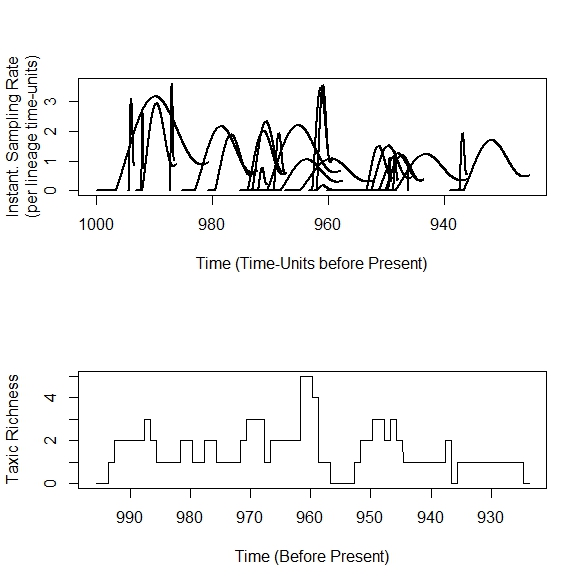
In this case, the 'hats' end up looking like they are sideways, as if
stylishly placed on one's head (with a chilling echo of Clockwork
Orange). This is because the interpretation of rTimeRatio differs when
per-lineage sampling rates are input, such that the input sampling rates
represent the per-lineage mean, thus requiring sampling rate to
increase over the duration of each taxon. The peaks of the hats can't increase like in the pull-of-the-recent+hat model above, so instead the whole hat tips forward. I realize that this somewhat different model behavior may seem undesirably, but there's a good reason for this: I want the models in sampleRanges to be collapsible: setting alpha=beta=rTimeRatio=1 will produce the simple Poisson model, because the input sampling rate is treated as the 'mean' sampling rate. If per-lineage sampling rates are used, this means the interpretation of what those sampling rates imply will be very different than when a single rate parameter is input for the whole dataset.
Including the hat model, pull-of-the-recent and among-lineage variation are good steps forward, but there are further expansions which can be made on these simulations of incomplete sampling. Holland and Patzkowsky (1999) presented a model where sampling was a function of preservation bias and changes in the sedimentary environment ('facies') producing the rock record with a depositional basin. Implementing a facies model of sampling in paleotree would be a lot of work, as it would require a model for simulating how facies are preserved within a given basin, but it would also be an important step toward realism. The produced fossil records would thus represent the observed sampling events in different sedimentary basins and several such records would have to be concatenated to produce a 'global' account of events. (So the number of basins sampled itself would be a parameter...). This would open up some incredible opportunities for understanding how the fossil record and the rock record should relate in a simple model (well, as simple as possible). What does sampling under the hat model, pull of the recent and facies-shifts look like? Are the fossil records produced by all these complexities even distinguishable from data produced by the Poisson model of sampling?
Finally, in other news, my paleotree paper just got accepted to MEE! I'll post here as soon as its up for download.