Friday, November 23, 2012

Playing Mountain Witch 11-21-12


I recently played a game of Mountain Witch which I would like to tell everyone about ! It was so amazing I must share!

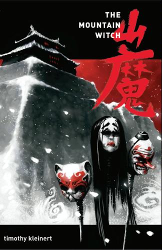
Stole this Amazon. Yeah, that's how I roll.
Obviously, I can only relate my account of events. It would be interesting to know what the other players were experiencing; there were certainly some bits I missed by leaving the room. I’m going to try to switch back and forth between what segments of the fiction which emerged and an account of the actual play.

We had Josh as GM and (if you don’t know Mountain Witch) the rest of us played ronin hired to take on the dangerous task of killing the powerful and god-like Mountain Witch. A fantastic wealth was promised to us if we could do this task. 

Justin playing Kagome (Dog, Yellow), who was a female samurai whose lord had been defeated in battle and who planned to kill herself after getting the money to completing some final task. Important to the game later, Kagome could smell fear itself and she had the preternatural skill to shoot anything she could smell. Alice played gray-haired Miyoko (Tiger, Silver) who was an older samurai who had become ronin after he made a reckless tactical mistake that led to his lord’s son dying in a rout, and hoped to reprove his loyalty with the reward money. Miyoko had a thousand shuriken hidden on his body and the ability to browbeat those who disagreed with him. Colin played Shigeru (Dragon/Green), a strong warrior who had willingly left his lord’s service, intent on raising funds for his own army and banner men, thus becoming his own lord. He had his armor and warhorse with him, which he rarely dismounted, meaning he often spoke down to the rest of us. Peter played Honzo (Red, Monkey), a man with plain features and red armor, who had been thrown out of his lord’s service due to an overheard insult. Honzo was a sneak, able to go where he liked without notice. I played Goro (Blue, Rat), a cynical man with sharp features who rumors say killed his wife and his lord after discovering them in a delicate situation. Blue tattoos covered his skin and he the ability to speak to birds and had a loyal crow who perched on his shoulder, Tsuba.

Note I only discussed a few of the powers, those I remember that became important to the fiction. Character creation was very good, we did powers like ala Settlers of Cataan town placement, where started at one end and then curled back around in opposite order (and then back again), so that there was some free equality in how powers were decided. It was probably unnecessary though, cause I think we each had very different ideas of what ronin powers should be.

An interesting thing which has happened is that there’s already been considerable drift in what I can remember from the game. Was Honzo shorter than the rest of us? Peter is somewhat short and as the game went on, he deliberately stooped in his chair, becoming even shorter. But I’m pretty certain Honzo started off at average height. I don’t remember if Colin described Shigeru as a giant, but that’s what he was by the end in my mind: a towering man of incredible strength. None of this was stated *I think*, and so I worry that means many of the things I say here may very much be not even have been part of the spoken narrative, but speaking with Peter suggests I was not the only one who saw these same shifts in our characters. Peter speaks of how Kagome became sterner and more like steel, how Miyoko became desperate and tired, more ferocious in his mission, how Goro (me) became more cryptic, solemn and quiet. I saw all of these things too in play, but I don’t think they were actually stated. Some of these shifts in appearance and personality (like my character’s) contrasted pretty strongly with the original characterization in act 1.

The first scene in Act 1 started with Honzo looking over at us and saying “Shall we go?” and starting our way into the forest at the base of the mountain. Soon we were in an encounter with wolves, which turned violent thanks to Kagome. Honzo and Goro stayed out of the fight, which ended quickly. Shortly after, a servant girl named Kono appeared from the forest, pleading with Shigeru to not kill the Mountain Witch. She claimed that both of them had once been in the Witch’s employ, but he refused to deal with her. Further on, the ronin had to cross a bridge in the forest and had to deal with the ghost of a warrior who had once followed Miyoko, but was browbeat by both Miyoko and Honzo to let them cross. Goro crossed on his own, leaping across the river. Kagome did not trust Goro and tried to follow, only to almost drown. Tsuba told Goro that Goro had to save Kagome, although Goro was angry that Kagome did not trust him. Still, he reluctantly had Tsuba drop a rope in the river to pull her in. 

All of the above had been framed by Josh, who then passed it on to one of us to frame, based on our dark fate. I volunteered and narrated us coming across a man holding his daughter, who was dead of mysterious cause. Kagome identified correctly that she was poisoned, having committed suicide in the same way as her mother. The father was distraught, and tried to kill himself with the poison to find answers to his daughter’s death. Miyoko considered this dishonorable and took the poison with her. Honzo, as he did repeatedly later in the game, claimed all of this was an illusion, trickery from the witch.

Next, we entered a place which Honzo later called the Vale of Dead Flesh, where we were attached by the restless dead, only to be saved by a magic word from Honzo. He claimed he knew this word because he had, in fact, been up the mountain to the Witch before but refused to explain how or why. The rest of the ronin presumed the word could only come from the Witch. We then came to a withered holy tree, tended by a spirit disguised a priest. Only Kagome considered herself worthy to go near the holy place, and it turned out the priest held a message for Miyoko. Kagome broke the sealed message open, to discover that it was from Ai, the former charge of Miyoko.  She was headstrong, and she was going up the mountain to face the Mountain Witch before us (maybe to save Miyoko from facing the Witch?). Following this, (Peter framing) we found a burial mound at a crossroads, which caused Honzo to freak out. Kagome shot it with her rifle and a severed child’s hand tumbled out of the mound. Goro recognized the hand and freaked out, but the hand vanished mysteriously in the ensuing chaos. 

At this point no one trusted anything: both Shigeru and Honzo appeared to be (at least former) servants of the Witch and Goro regularly whispered things to Tsuba in bird-tongue who would then fly away and return some time later. Miyoko and Kagome were fast relying on each other as the only two trustworthy members of the ronin. Shigeru constantly tried to deflect suspicion on himself by questioning the motives of Honzo and Goro. Goro was adamant that his goal was to kill the witch and Honzo was equally adamant that his goal was to complete ‘the Mission’. 

Kagome did not trust either Goro or Honzo. As the group crested a hill, she whispered to herself that she had smelled no fear yet on one of the men she travelled with, and that her mission would be to kill the Witch, but also to make this man feel fear and kill him.

We camped (end of Act 1), taking turns at watch. There was a scene I wasn’t in the room for, where I think the Witch invaded the dreams of Miyoko and/or Kagome, and there was something involving the bottle of poison (??).  Later in the night, during Goro’s watch, which Kagome forced him to share with her, Kagome saw him conversing again with his crow, who flew off, up the mountain.
Trust point change time! It was clear Kagome didn’t trust Goro, and I reciprocated by dropping trust points with Kagome down to one. I increased Goro’s trust for Honzo, but I was the only one, and Miyoko. Overall, much trust was lost for both Honzo and Goro.

In the morning (now Act 2), the warriors were greeted by a friendly 40 foot tall rock giant, who claimed he was the chancellor of the Witch. No one trusted him. He gave the ronin a bundle of food and passed on a message from the Witch, who politely suggested they should give up their mission. He also deposited a bundle of gold, a gift for the true servant of the Witch among the group. Only Shigeru touched either of these bundles, taking some food while the others were leaving. Goro told the chancellor to tell the Witch that nothing would turn Goro from his task. As the ronin walked off, Tsuba flew back, snatching a note hidden among the Chancellor’s gold. The crow gave it to Goro who read it and tried to throw it away in a sudden fit. Shigeru grabbed the note with his spear and read it: it was “Kikuya”, the name of Goro’s dead wife… and a name which Miyoko had heard Kagome utter in her sleep last night. Tensions between Goro and Kagome almost peaked, but Kagome won the staring match. Goro came away only knowing she knew… something about his wife.

We came to a crossroads, where we could travel either by tunnels or by the precipice road, and Kono appeared to plead with Shigeru again and declaring her love for him, asking him to think of the things the Witch had done for both her and Shigeru. Shigeru (or someone) threatened to kill her if she did not leave. Taking the precipice road, the ronin were faced with ice demons and their fierce winds, who tried to shove them off the mountain. Goro sliced the wave with his sword, but Tsuba was grabbed by the wind and flung off far down the mountain (I narrated this). Both Honzo and Shigeru lost their footing and nearly died, but Honzo used another magic word and Shigeru called on the Witch to honor their deal. Having survived, the ronin quickly made it to an inviting cave where Honzo and Shigeru might have been interrogated if the cave wasn’t already occupied (I framed). An old man sat by a campfire and offered to tell samurai a tale as they tended to their wounds and dried out by the fire. He told of an emperor in a far off land, who realized he was disliked, so he made himself so hated that his people stormed the palace and killed him, but he had last laugh because- at which point in the story, Goro sliced off the old man’s head and covered Shigeru and Kagome with blood.

The ronin exploded into distrust, with Shigeru trying to deflect suspicion on himself by instead trying to claim that Goro and Honzo must be spies of the witch. Honzo’s sanity was clearly slipping and Peter was fantastic, stooping to look smaller and smaller, grinning and mumbling constantly about how they had to complete the Mission. The nearly violent dynamic between Colin as Shigeru (who grew somehow to be a giant samurai full of arrogance and bluster) versus the impish and unwell Honzo was probably the most memorable part of the game. It was clear Honzo had been up the mountains many times and Goro seemed to withdrawl emotionally following killing the old man, becoming ever more solemn and cryptic, only being adamant that they must kill the Witch. Honzo seemed to have almost become a risk but his clear experience with the mountain path was too valuable to force him from the group. Goro asked Honzo if he was the ‘next one’ but Honzo had no idea what Goro was talking about.

Miyoko seemed the most sane of the ronin, but not for long. Travelling on, they found a scabbard for a woman’s sword, which Miyoko remembered giving to Ai. It was clear that a struggle had occurred here but there was not trace of Miyoko’s former student. He became obsessed with moving on to the palace and making sure Ai did not die like the men who Miyoko had once led to their doom. As they entered the volcano, they snuck past several trolls, preparing a mortal for dinner. Honzo recognized the man as his former lord but was completely indifferent to this emotionally, stating that it was clearly another illusion. 

The ronin made their way down to the Witch’s stronghold, to the bridge which marked the edge of his demesne. There, Kikuya’s ghost appeared and warned her sister, Kagome, to not trust Him, and she seemed to not notice Goro’s presence at all. Goro went into emotional trauma again, begging Kikuya for answers: was she having an affair with his lord? Had their deaths been righteous or not? Did she forgive him for what had happened to their daughter? No response and the ghost left having given its message to Kagome. Suddenly, as if a spell was broken, Goro could see that Kagome was nearly identical to his dead wife. He begged Kagome to forgive him, that he had thought Kikuya was keeping something from him, that he was sorry that he had killed Kikuya.

 Kagome informed him that he hadn’t killed Kikuya… Kagome WAS Kikuya! The two sisters had switched their names when Goro had become arranged as ‘Kagome’s husband-to-be, so that Kikuya was spared the harsh life of a woman samurai. Goro was in tears, as ‘Kagome’ told him that they would kill the witch, but then she would kill him for the death of her sister. Goro, suddenly angry, told Kagome that the only thing that mattered was that the witch must die.

Trust points continued to evaporate and cluster although I can’t remember all the details. Goro trusted Honzo and Shigeru highly (4 and 3) to kill the witch, but both of them could not trust him nor each other. Miyoko continued to trust Goro somewhat (2) and Kagome (who had been saved repeatedly now by Goro, but also intended to kill him) gave Goro a single trust point. Goro trust Miyoko also to kill the witch, but could not trust Kagome, knowing that Kagome meant to kill him. Miyoko and Kagome continued to be bound tightly in trust. I think trust evaporated for Honzo completely except for Goro’s trust, and the same for Shigeru.

At the start of act three, Tsuba reappeared, landing on Goro’s shoulder, where he told Goro that the shadow puppet was ready. Goro nodded. The ronin entered a great plain before the Witch’s mighty fortress, only to face an army of several thousand vicious Oni. In the face of great and violent death, the ronin ran, with Shigeru taking lead and pulling a note from his armor with a map of the fortress on it. The oni pursued with no mercy. Miyoko tripped and Kagome tried to help him, only for Goro to grab both of them from behind and pull them up. He told Kagome he had no intention of letting the real Kikuya die also. At a shear cliff wall, Shigeru uttered a magic word which opened a secret entrance to the Witch’s library and then sealed it after the other ronin stepped through, saving everyone from death. Goro wondered where the note had come from, and the crow whispered that he’d given the note to Shigeru. (In play we knew it came from the Witch, and there was some confusion when I said that the crow had told me this. I think some thought I was making a joke. I was not.) Shigeru explained he had once worked for the Witch but he was now completely devoted to killing the witch.
In the library, Honzo began leading the ronin through hallway after maze-like hallway, searching for the book of souls. Shigeru and Goro separated from the others, with Kagome following Goro refusing to let him be alone and contact the Witch. She was now convinced that Goro was the servant of the witch. Miyoko stayed with Honzo, who Kagome and Miyoko agreed was much more dangerous than Shigeru.

 (Colin narrating) Shigeru, by himself, wandered to an isolated section, where he pulled out a hand mirror. The hideous visage of the Witch formed there, and told Shigeru that he had done well, having brought the ronin to the stronghold so that the Witch might absorb their souls. Shigeru thanked his lord and saw a vision of the vast wealth and mighty kingdom he would rule as his reward. Shigeru added that he wanted his love (Kono?) by his side. In play, there was an odd bit here where several of us rechecked our Dark Fate cards. I had some pretty complex narrative plans in particular, and I felt somewhat impatient to have my own dark conference with the Witch to clarify what I’d been hinting at all game-long. It wasn’t going to happen though, not with Kagome around. I just had to take solace in the fact that I knew my Dark Fate gave me the end-all-be-all narrative control over the elements of my own Dark Fate and that I’d be able to tie my outlook in eventually.

Honzo found the tome of souls (he knew exactly where it was already, having been there before). It was a giant book, bound by chains and lightning. It could kill any mortal who touched it. Honzo was unharmed as he leafed through it, because he had no soul and proceeded to look for the entry that would tell him where his soul was. It was in the Witch’s throneroom. Miyoko requested desperately if they could go to the dungeon, where perhaps Ai was being kept, but Honzo informed him that he had looked up Ai in the tome and she was also in the throne room. 

Meanwhile, Goro revealed all to Kagome: He had killed her sister and his lord in a moment of passion, believing that they were cheating behind his back, and that then he had run in cowardice. In absentia, Goro was punished by his lord’s family by his daughter with Kikuya being executed. His sin knew no end, but he could make it right. He asked Kagome to trust him: if the Witch died, ‘Kikuya’ would be returned to this world. Kagome said she would help in killing the Witch, but Goro would die soon after if there was any treachery. Goro conceded to this. Shigeru, Miyoko and Honzo reappeared, at which Goro tried to sneak away. It was almost too easy for Kagome to shoot Goro through a bookcase, leaving him wounded and unable to get away. He was not, would not, be out of Kagome’s sight again.
It was at this point that Josh said he knew what all our dark fates were. He was mostly wrong. I don’t think any of us knew who the others fates were.

We made our way through the palace until we got to the hall of crystals, the anteroom to the throne room. (Alice narrating) Miyoko glanced in one crystal and suddenly was back as the master samurai, teaching tender Ai the art of the blade. His soul began to leak out into the crystal and Kagome grabbed him, trying to tear his gaze from the crystal, only for her own eyes to fall on one. (Justin narrating) Kagome saw an image of her and her sisters as happy innocent children, but she pushed this to the back of her mind and saved Miyoko. (Colin narrating) Shigeru looked and could only see his anger and jealously, how he had seen the riches of the lords and how wanted them, particularly the love they received. He would lead the rest of us to our deaths and take all of the wives of his former lords as his own. (Peter narrating) Honzo walked through unimpeded, for he had no soul.
(I narrating) Goro looked at the crystal and saw first himself, as a samurai. He had led his lord’s men to victory, and there was a grand celebration. Then he looked over and saw his wife and his lord talking quietly. Goro’s heart darkened at that moment. He always knew his wife held something from him, had some secret she would not tell him. Was it that she did not love him, maybe loved another? Then the vision changed, now it was later, after Goro had killed his wife and lord in anger and killed his daughter in cowardice. It was now the throne room of the god-like Mountain Witch, with the mighty monster of ice and fire that was the Witch sitting on his throne. A ruined man was dragged in by Oni, “We found this one trying to commit suicide in the forest below!” they cried. Let me die, Goro pleaded. The Mountain Witch laughed and offered to undo Goro’s sins. The Witch told Goro of the Emperor’s tale, this time including the ending: that the hated emperor had arranged for a double and so it was not the Emperor that was killed. Instead, the hated Emperor had abandoned his life as a disliked ruler and escaped to die at an old age, as a happy and fat peasant. The Witch wanted to do the same: he no longer wished to be hunted and hated but instead to leave his power and trapping behind. So, here was the plan: the Witch had selected several powerful ronin and Goro’s task was to lead them up the mountain. They all had their reasons to hate and despise the Witch and he would give them even more, except one, who he had groomed to be the Witch’s replacement, to become the next Witch. All Goro had to do was help the Witch fake his own death and destruction.

Finally, the visions faded and now it was a reflection of Goro, but the thing on his should was not his crow, was not Tsuba, it had never been. It was the Witch. The Witch had been with the ronin as Goro’s crow the entire journey. The thing that sat on the throne in the next room was the shadow-doll, ready to be slaughtered. 

We entered the throne room (no one shifted Trust), and saw the giant Witch-Shadow-doll of ice and fire sitting on the throne. Ai was trapped in a block of ice, forced to dance for his enjoyment. Miyoko stepped forward and battle commenced, with Honzo immediately running off to look for his soul among the witch’s treasures. Shigeru went after him (I think?), because he needed all of our souls to be absorbed into the Witch (or was it the shadow puppet? was the witch lying to someone? there was still doubt here for us at the table about who knew the truth of the situation). I cannot remember what Kagome was doing during this portion, but I know that Miyoko and Goro fought the ‘Witch’, with Goro eventually distracting it while getting burned by fire. The distraction worked long enough for Miyoko to kill the god monster, filling throne room with a rolling cloud of steam and melted ice. The crow cawed and Goro dropped his blade. The bird took off down a distant hallway, past piles of treasure and wealth. Goro followed, followed by Kagome, readying her rifle.

Miyoko strode forward and dug Ai out of the melting ice, making sure she was okay. Shigeru, full of rage and fury that the Witch was dead, attacked Miyoko and the two dueled as Ai watched helplessly. It ended with Miyoko’s shuriken in Shigeru’s eye, his blood seeping out into the melted water that had once formed the ice-body of the Witch/shadowdoll.

Far off in a distance section of the throne room, Honzo found the pot with his name on it, opened it and… it was empty. Suddenly he remembered, very briefly: he had no soul. He never had! He was just a creation of the Witch’s, given memories as a toy, a plaything, an eternal traveler who would forever gather ronin and then shepherd them up the mountain to the stronghold, while he looked for his soul. And then… poof, Honzo simply stopped existing.

Meanwhile, the crow landed on a giant clay pot, next to two other giant pots. The bird cawed several instructions to Goro and then flew off to freedom, out a window, supposedly to a new life where it was no longer the Witch. Goro smashed the pots open: within one was his former lord, within the second was ‘Kikuya’/the real Kagome, and the third held their daughter. Each pot was also full of rice vinegar, and as each spilled out, they coughed and began to breathe. The witch had kept his promise: this was Kikuya and the others truly returned to life. The samurai known as Kagome ran forward to cradle her sister. Goro begged for forgiveness… he no longer needed her to return to give him answers, he knew now, thanks to Kagome, what secret she had been keeping. 

But even in this moment of happiness, some sins cannot be fully undone, some things cannot return to how they were. ‘Kagome’ would not take her revenge, she would not kill Goro. But she did force Goro to leave, to turn his back and never come near her sister or niece ever again. His reward and other riches for killing the Witch would be split between his wife and his lord, now returned to life, to make up for his crime. 

Our epilogues are great, and I’m gonna do a bit of curating here in the order I report them. This is not the order we narrated them.

Miyoko returned to his former lord and begged forgiveness, giving his lord his money, and finishing Ai’s training.  Kagome, once she had made sure that her sister and niece were well taken care of and that Goro would never come back, killed herself, following her fallen lord into the afterlife. Goro left and never picked up a weapon again, living a lonely life as a monk, but knowing some peace in that his sin was undone and his family lived once more.  At night though, he would hear a crow and wonder if perhaps he had replaced one crime with another. 

In the throne room below, the water the shadow puppet was made of began to freeze again, reforming, only now Shigeru’s soul was pulled out his dying body, his blood intermingling, his flesh changing. He became the new Mountain Witch, with all the power and riches he had ever wanted, all the maidens and wives he could ever desire, but trapped in a body of ice and fire with no escape and no way to love another.

Tsuba, i.e. the crow, i.e. the Witch, flew around the stronghold several times after the ronin left, then flew into a tiny room at the top of a tower. Kono sat there and the crow landed on her shoulder. “Again, again!” she cried. “Let’s do it again!”

Then, at the base of the mountain, we see an average looking man with plain features, wearing red armor. He glances over a group of ronin he is with. “Shall we go?” he says to them.

.....
 
With the game over, we revealed all of our dark fates. As may be apparent, none except Honzo’s and Kagome’s had been absolutely clear up until then: Honzo had the other mission, Kagome was revenge, Shigeru was Love, Miyoko was Loyalty and Goro was Unholy Pact. From what I understand, Josh’s guesses were mostly off. Somehow, and this wasn’t intentional, most people had become convinced my dark fate was love.

So, some thoughts.

So, my biggest takeaway, the one that hit me after playing it was how cohesive the story was at the end. Normally, improv and sharing narration is great but… in my experience, someone always bends a little to silliness somewhere or we all forget some plot thread and stuff is left unanswered at the end. I don’t play a terrible lot of narrativist games, but this is just something I’d accepted a side-product of allowing shared narration. I didn’t really get that this time. I don’t know exactly why, maybe it’s cause narration with respect to our dark fates was inviolate. Maybe other players felt differently, but I look back on what I just wrote here and its just freakin’ incredible how cohesive and amazing all of it was.
So, I think I’d laid enough clues that my little spiel in the crystal room wasn’t a crazy sudden plot punch from the right, but at the same time Kagome hadn’t given me many options to reveal this narrative twist. (Just how should an Unholy Pact-man expose his status to the players and not the characters when one character was watching him like a hawk?) To be honest, I had been laying the foundation for this twist since Act 1. I’d be interested to know how much of a shocker this was from the other players. All I know is that I knew that I considered this my narrative claim as I had the Unholy Pact as my dark fate: this was the deal the Witch had made with Goro. I think that having the Dark Fate as your own thing that no one could mess with was really awesome because it let me.

Now, here’s a thing… I could only explain Colin’s narration as Shigeru being kind of set-up by the Witch (and, let’s be honest, the things the Witch was promising Shigeru fit rather well with an interpretation that Shigeru was to become the replacement Witch). I was really trying hard to make it so it didn’t de-protagonize him and that just seemed the best option. Becoming the Mountain Witch is pretty awesome, well, to me at least.

The way it worked out, I was very glad that it had been unable to get exposed until right before we entered the throne room and it worked out wonderfully, but that sort of 20 ton thermonuclear plot bomb so close to the climax could have gone so very badly in many other games. I also wouldn’t do a twist where the Witch’s unholy pact was to get killed again, but I think this one time it really worked out well.

Most of us had not played Mountain Witch before; I don’t know really if anyone had played it before other than Josh. I hadn’t, I had just wanted to (and to read it… speaking of which, Kleinart, I can’t wait to buy the next edition now.). Josh, Peter and I were fairly familiar with narrativist story games. Colin and Alice were new to these types of games. I do not know Justin’s background. We made pretty good use of the rules. There was A LOT of fishing (AKA the Mountain Witch trick, i.e. the GM asking leading questions). So much fishing! Fishing was probably more common than Josh actually just making statements of narration. And it all worked out pretty great. In terms of the mechanics on the sheet, we didn’t make a lot of use of some of them. Betrayal came up, but only once or twice. We never(?) stole narration from each other, I think. There was a lot of aiding throughout the game.

So, anyway. That session was freaking incredible.

Thursday, July 26, 2012

Resolving Polytomies According to Temporal Order

Hello everyone!

A user of paleotree recently asked about resolving non-bifurcating nodes according to the order of stratigraphic appearance. If you're familiar with the library ape, you know there's a function called multi2di, which resolves polytomies randomly into bifurcating nodes. But what if we want to include information we have about WHEN taxa show up in the fossil record, assuming that taxa which show up later are more likely to be closely related?

My library paleotree has the Sampling Rate Calibrated time-scaling methods (SRC timescaling), which will resolve polytomies according to a probabilistic approach about gaps in the fossil record. This function can allow for ancestor-descendant relationships, although that aspect can be shut off or minimized to the user's discretion. However, how SRC methods work and whether it works well isn't something that's known to anyone but me, (maybe) my committee and whoever has asked me about it. Also, it needs an estimate of sampling rate, which isn't always obtainable.

So, as another option for resolving polytomies, I've made a new function called timeLadderTree, which takes polytomies and turns them into little pectinate (ladder-like) sub-trees. Each lineage in the pectinate sub-tree is ordered according to the time of first-appearance datum (FAD) for each lineage, for both clades and single taxa. This method of resolving polytomies assumes that the order of stratigraphic appearance perfectly depicts the order of branching. This may not be a good assumption for poorly sampled fossil records, but hey, maybe it's still better than assuming a completely random solution for a polytomy.

I'd paste the code here, but it's really long. If you really want it, email me or you can get this function either from the public paleotree library source file on github, which I'm pushing to as we speak, or just wait until the next paleotree release (sometime in the next month). Also in the newest release, I'll be including this function as an additional option for timePaleoPhy and bin_timePaleoPhy to resolve the tree with. The new argument will be called 'timeres' and setting it to TRUE will cause trees output with those functions to have polytomies resolved according to time of first appearance. (Obviously, this is incompatible with also setting the argument 'randres' for random resolution via multi2di to TRUE and doing such will return a warning).

Okay, so how does it work? Well, let's say we have data and some stratigraphic ranges that look like so...

...And we get a nice pectinate tree.

What that poorly-scrawled M$Paint image means is we need a tree in R (in 'phylo' format) with polytomies and a set of temporal data, in timeData format as is standard for taxon ranges in continuous time in paleotree. timeData matrices look like the following, where row-names are the taxon names.

            FAD         LAD
t1   170.391157 147.8839782
t2   158.519694 152.6571314
t3   149.415686 128.5232837
t4    ...                  ...

Note that this function is for resolving tree when a continuous time-scale is known. For discrete time-scales, where appearance dates are known from intervals rather than from specific points in time, users should use the function bin_timePaleoPhy, which stochastically produces arrangements of dates in discrete intervals in the course of time-scaling. This would be the preferred way of doing things with datasets where taxa are known on discrete time-scales (most data in paleontology, probably...).

You might wonder how this function handles ties. Well, taxa with the same identical first appearance date will be ordered randomly. Thus, the output could be slightly stochastic (it'll differ each time you run it), but this only occurs when taxa descended from the first node have the same first appearance datum in continuous time exist. This is probably uncommon with real data on continuous time-scales. Thus, resolving polytomies based on time-order will probably produce a single same tree each time you use it, unlike multi2di which is guaranteed to not produce the same tree each time. It's a pretty strong assumption though, to make, that order of appearance perfectly predicts branching order, though!

Because simulating clades in paleotree often produces partially unresolved trees (for reasons I explained last time) we can test this function pretty easily.

library(paleotree)
set.seed(444)
taxa<-simFossilTaxa(0.1,0.1,mintaxa=100)
tree<-taxa2cladogram(taxa)
ranges<-sampleRanges(taxa,r=0.5)
tree1<-timeLadderTree(tree,ranges)

And we can see the difference in our two trees, with the second have some very pectinate-looking regions...

layout(1:2)
plot(ladderize(tree),show.tip.label=FALSE)
plot(ladderize(tree1),show.tip.label=FALSE)
(Apologies for all the white-space, I didn't crop this one before pasting it...)

As always, let me know if you have any new ideas for paleotree that you would find useful in your own work!
-Dave

Tuesday, May 1, 2012

Simulating the Fossil Record: Incomplete Sampling and Hats

Alright, here we go for part 3 of my series on simulating in the fossil record. If having explicit models of how morphological differentiation evolves in lineages is critical to understanding observed patterns of diversification in the fossil record, than the second major difference is incomplete sampling. Sampling issues are important to every field, but paleontologists and geologists has always been especially concerned with accounting for the incomplete and gap-filled nature of the fossil record.

To appropriately model the sort of data we generally have in reality, simulations of diversification as observed in the fossil record must consider some model of incomplete sampling. In continuous time, the simplest model treats sampling events as a Poisson process, just as the simplest models of speciation and extinction treat those events as Poisson processes. Under this model, the waiting times between events are exponentially distributed with some instantaneous per-lineage-time-unit rate parameter, generally called r (Foote, 1997).

(Tangent on terminology: r matches alright with the general paleobiological usage of p and q for speciation/origination and extinction rates, but not so much for the biological usage which uses lambda and mu for those same rates. Stadler (2010), however, defined sampling rate as a variable (independently possibly, given no references to the paleontological literature) and used psi. For me, though, it'll always be lower-case r.)

Here's an old figure (I need to heavily revise it) from my in-the-works paper on time-scaling methods which illustrates sampling in the fossil record:


As in previous similar figures, (a) is the original ranges and relationships of some morph-taxa, (b) is one possible outcome under a Poisson-process sampling model and (c) are the temporal ranges we would recover for those taxa we sampled, in continuous time (more or less; F should be a one-timer). (d) is a tangential bonus, just showing what sort of relationships we would resolve among the sampled taxa using morphology-based cladistics (see the last post for why there is a polytomy.)

As we can see in this simple model, incomplete sampling slices the early and later parts of a taxon's history off, if that taxon is sampled at all. In continuous-time, a majority of taxa will probably have zero-length observed durations ('one-timers'; Foote, 1997). In general, longer-lived taxa will be more likely to get sampled at all and to have positive-length durations, so the probability of sampling any given taxon is not the same.

There are a number of additional complications in how taxa are sampled in the fossil record which make this Poisson model of sampling in continuous time unrealistic. Generally, the ability to temporally resolve the 'date' that any particular taxon is sampled is not so great, and can have considerable error bars. This is generally done with relative dating, using 'biozones', where time is defined based on the appearance of zonal taxa (graptolites happen to be great for this purpose). In some cases, these can be well resolved temporally by correlation with absolute dating (Sadler et al., 2009), for example, Sadler et al. presented global graptolite zones a few hundred thousand years long and for which the start and end dates can be resolved within a few thousand years. However, biozones tend to not extend to the global level and even then the appearance of taxa tends to not by synchronous globally (Sadler, 2011; Loydell, 2012). Some taxa are better than others for defining short biozones. If your Ordovician rocks only have corals, for example, it might be very difficult to correlate those globally with precision, unless other information is available.

Geologists have constructed hierarchical time-scales with eras, periods and stages, all rigorously defined (or proposed to be) based on particular 'type sections', just as Linnean taxa must be based on type specimens. Although we now have global-level systems for much the Phanerozoic (the last ~500 Ma), with the starts and ends of intervals attached to the boundaries between bio-zones, many finds from previous decades are still only reported in terms of more regional systems of intervals, which can be very difficult to correlate to the global system. Thus, in general, our finds are really known from more discretely known intervals, and the order of events within a given interval may be very difficult to resolve. (e.g. A find of Normalograptus normalis within the N. extraordinarius biozone could come from anywhere within the N. extraordinarius biozone.)

In general, a way to deal with these additional complexities of how the nature of correlation and time-scaling of the rock record itself works is to impose a system of discrete intervals on a set of continuous-time sampling events. I think this makes the most sense, as we generally simulate branching processes as the result of instantaneous rates, we should speak of sampling in terms of an instantaneous rate. Some previous studies placed lineages, generated in continuous time, into a discrete time framework and then sample them within those intervals under some per-interval sampling probability. However, the relationship between the instantaneous sampling rate (r) and the per-interval sampling probability (R; Foote and Raup, 1996) is not exactly simple, although it can be loosely approximated (see the function sRate2sProb in paleotree). The per-interval probability assumes taxa span the entire interval, which may not be true as average interval length increases relative to average taxon duration. Also, the discrete time intervals are imposed secondarily by us, the geologists, and so it just makes more sense to me that we should simulate sampling on lineages in continuous time first.

Simulating sampling originally in continuous time actually allows for very quick simulations of sampling. simFossilTaxa makes use of the Poisson process nature of the processes it simulates to only consider the waiting times between events. Its sister function, sampleRanges, does the same thing by default, pulling the waiting times for sampling events from an exponential distribution. It is then very simple to apply binTimeData to the output from sampleRanges, which produces (by default) ranges placed into intervals of equal length, but (as of version 1.3) allows for user-input ranges as an alternative. A future modification may allows for intervals to be defined based on the origin/extinction of taxa, which would be more realistic as the real discrete intervals of the geologic record are often based on such biostratigraphic events (for example, periods were often defined with mass extinctions placed at their boundary, as this created a considerable amount of faunal turnover that allowed for biostratigraphic dissection).

For example, we can simulate sampling on example dataset from the R help file for sampleRanges, with the sampling rate set to 0.5 per Ltu (lineage*time-units). The flat line at top is the (unvarying) sampling rate over time and below it is a diversity curve produced from one simulation of sampling.
However, we may want to go further. Liow et al. (2010) represented an important step forward in the field of 'simulating diversification in the fossil record' by allowing for very complex sampling models, which went beyond the 1-parameter Poisson model. The newest version of paleotree includes a greatly updated version of sampleRanges which includes these models.

For example, we might think that as we get closer to the present, more of the rock record is available and preservation is better so we are more likely to sample taxa. A very simple model of this would be a linear increase in sampling rate over time.

We can simulate this by changing the parameter rTimeRatio, which is basically the increase over time from the start of a clade's origin to its end. The input sampling rate becomes the mean sampling for the dataset in this case (the sampling rate observed at a clade's midpoint. For example, here is a plot of sampling rate for a clade varying over time when rTimeRation=5, along with the observed diversity curve produced by simulating sampling under that model. This plot can be easily reproduced with the examples code in the sampleRanges help page in paleotree 1.3, by the way! You can go run it yourself!

Another model is the 'hat'. Various studies in the last half-decade have suggested that taxa tend to be most abundant and geographically wide-spread in the middle of their geologic duration: the rise and fall of species and genera .  Also remarkably, this rise and fall looks like a remarkably normal-looking symmetrical curve. (Lee Hsiang Liow tends to refer to this as the "hat" in her work.) This would lead one to expect that perhaps the rise and fall of taxa might also influence sampling, such that the probability of sampling is highest in the middle of a taxon's temporal range.

sampleRanges can handle this by changing the alpha and beta parameters: when they are set several times higher to 1 and are equal, you get a bell-curve-looking symmetrical distribution. Here, with alpha=beta=4, we get the following, with taxon range represented by a single symmetrical 'hat' of sampling rate increase and decreasing over its range. Again, the sampling rate input (0.5) becomes the 'mean sampling rate' for the dataset.

(A stray thought: presently, the shape of the hats are dependent on the taxon range, such that simulations with some extant taxa will have those taxa decrease in sampling rate as their range appears to 'end' at the modern. Hmm. But what would be more realistic? Choosing how 'far' they are with their hat at random using a uniform distribution or placing the peak arbitrarily at the modern? Hmm.... something to think about.)

But what if sampling increases absolutely with time AND there is a general tendency for better sampling in the middle of a taxon's range? If we force sampling to always be zero at the end of each taxon's range (as its range gets smaller and smaller...) we would expect this to look like hats which are growing bigger in size as time goes on. If we set rTimeRation=5 and alpha=beta=4, we get...

Finally, the new sampleRanges also allows for among-lineage variation in sampling rate. For example, we could imagine traits which determine sampling rate (such as shell thickness) increasing and decreasing as a trait evolving under Brownian Motion. An example of this is also included in the sampleRanges help examples and produces a pattern sampling rates which looks like:

sampleRanges can go one step further and even consider a model where lineages vary in their intrinsic 'mean' sampling rate (on a per-lineage basis), have 'hat' shaped sampling rate curves AND sampling rate is overall increasing over their duration.
In this case, the 'hats' end up looking like they are sideways, as if stylishly placed on one's head (with a chilling echo of Clockwork Orange). This is because the interpretation of rTimeRatio differs when per-lineage sampling rates are input, such that the input sampling rates represent the per-lineage mean, thus requiring sampling rate to increase over the duration of each taxon. The peaks of the hats can't increase like in the pull-of-the-recent+hat model above, so instead the whole hat tips forward. I realize that this somewhat different model behavior may seem undesirably, but there's a good reason for this: I want the models in sampleRanges to be collapsible: setting alpha=beta=rTimeRatio=1 will produce the simple Poisson model, because the input sampling rate is treated as the 'mean' sampling rate. If per-lineage sampling rates are used, this means the interpretation of what those sampling rates imply will be very different than when a single rate parameter is input for the whole dataset.

Including the hat model, pull-of-the-recent and among-lineage variation are good steps forward, but there are further expansions which can be made on these simulations of incomplete sampling. Holland and Patzkowsky (1999) presented a model where sampling was a function of preservation bias and changes in the sedimentary environment ('facies') producing the rock record with a depositional basin. Implementing a facies model of sampling in paleotree would be a lot of work, as it would require a model for simulating how facies are preserved within a given basin, but it would also be an important step toward realism. The produced fossil records would thus represent the observed sampling events in different sedimentary basins and several such records would have to be concatenated to produce a 'global' account of events. (So the number of basins sampled itself would be a parameter...). This would open up some incredible opportunities for understanding how the fossil record and the rock record should relate in a simple model (well, as simple as possible). What does sampling under the hat model, pull of the recent and facies-shifts look like? Are the fossil records produced by all these complexities even distinguishable from data produced by the Poisson model of sampling?

Well, that ends this series of posts. So, who is excited to simulate the fossil record? I know I am! I love being a paleobiologist because I get to sit around and come up with fun toys for simulating the fossil record. :D

Finally, in other news, my paleotree paper just got accepted to MEE! I'll post here as soon as its up for download.

Sunday, April 29, 2012

Simulating the Fossil Record: Cryptic Species, Phylogenies and Resolvable Clades

Okay, so let's pick up where we left off with a small tangent.

First things first: I released a new version of paleotree, version 1.3! It has a number of new elements, particularly one item I will talk to you about today: cryptic cladogenesis.

In the last missive, I argued that any simulator of "diversification in the fossil record" had to be enmeshed with some assumptions (i.e. model) of how morphologically distinguishable taxonomic units arise, as these are the basic units that we (paleontologists) can identify, relate and measure. These morphologically-deliminated, sometimes temporally-extensive units can represent something very different than equivalent taxa in evolutionary biology (Forey et al., 2004; Ezard et al., 2012).

To clarify some of my explanations last time, it may be helpful to think of two general classes of events. First, one could have 'anagenesis', where a lineage experiences a morphological change that is geologically-sudden, producing a new 'descendant' morphotaxon distinguishable from the previous 'ancestor' which no longer appears. As we generally define and distinguish taxa based on discrete or meristic characters, like the presence or absence of spines, one can think about these events as the change of one or more such characters. If they ever change again, then that would be another 'anagenetic' event and another new morphotaxon would origination, and so on.

(Note that this is different from how most people define anagenesis! Most of the literature using this term is referring to changes in continuous traits, particularly traits which don't (generally) get used to distinguish taxa. I'm only interested in shifts between recognizable morphotaxa, so I'm limiting my usage of anagenesis to describe that and being totally agnostic to how non-systematically-informative traits vary within lineages.)

Now let's think about how branching events, cladogenesis, comes into this. Let's limit ourselves to only bifurcating events, which produce two daughter lineages. We can contextualize the 'bifurcating and budding cladogenesis' of the last post by considering these as all part of a system of whether morphological change must happen in one, both or neither of the daughter lineages. Like so:

In cryptic cladogenesis, both daughter would continue to be diagnosed as the same morphotaxon as the ancestor, in budding one of the daughter lineages becomes a new morphotaxon while the other experiences no morphological shifts, while in bifurcating cladogenesis, two new morphotaxa arise and the ancestor no longer exists. We can describe any model of how distinguishable morphotaxa arise in the fossil record as some mixture of these four event classes (anagenesis, cryptic clado., budding clado. and bifurcating clado), which even more simply can be described as 'shifts within branches and shifts at branching events'. If we can describe these processes in a model, then we can include most previously described models of morphological differentiation, at least the ones described for processes on geologic timescales.

The function simFossilTaxa can simulate all of these and any mixture of these processes, within the (generally assumed) constraint that diversification and the morphological shifts occur as Poisson processes. The big major change I had to do to allow for cryptic cladogenesis in paletree 1.3 was a new column which describes which morphotaxon each lineage would be assigned to (due to being functionally identical).


With this new feature, we can do fun things like simulating only under cryptic cladogenesis and anagenesis. This gives us patterns like these, using a particularly relevant example.


Okay, now, this post is supposed to be about how we can turn simulated data from simFossilTaxa into cladograms and phylogenies, using the functions taxa2cladogram and taxa2phylo. Just how does paleotree do that, really?

Well, check out this figure that I totally wish I had room for putting in my MEE submission on paleotree.


So, let me walk you through this. In (a), we have three morphotaxa, related to each other by budding cladogenesis and (b), (c) and (d) are various phylogenetic interpretations of that data.

In particular, (b) is the result of transforming such a dataset into an uncscaled cladogram with taxa2cladogram. This is an unscaled set of nesting relationships (i.e. clades), containing all the clades that could be resolved with morphological data, assuming that shifts in systematic characters can only occur when new morpho-taxa originate. (This is a pretty good assumption: if we see shifts in systematic characters within a lineage, we generally start calling the critters a new name in the fossil record!) The distinctions between morphotaxa are captured in all that information output by simFossilTaxa.

Note that in this case, you get a polytomy. For cases where there is a single ancestor, static in systematic characters and multiple descendants via budding cladogenesis, you get a polytomy, which was originally shown by Smith (1994) and Wagner and Erwin (1995). This is true if you sample two descendants and an ancestor or just three descendants. You can also get it if you have bifurcating cladogenesis and sample ancestors. You will end up with more than two taxa that contain no actual synapomorphies, although in practice this would actually look like either some poorly-supported relationships (on a set of most parsimonious trees) or a polytomy (on a consensus tree).

I've been looking at this issue in great detail lately, with respect to varying how shifts occur under the various models of morphological differentiation we've discussed and with varying rates of sampling in the fossil record. I've decided to write this up as a chapter for my dissertation, so I can't say much at the moment, but the short answer is that it could be a very serious issue: some simulations have have very few resolvable clades at realistic sampling parameters.


Now, (b) and (c) are a little more complicated, representing different ways of translating (a) into time-scaled phylogenies using taxa2phylo. The first thing to understand is that there is no such thing as a single time-scaled tree that will describe the relationships for lineages that span intervals of time. None!

All we can do is talk about the relationships about populations at particular points in time. We might want to do this, for example, if we want to simulate continuous traits evolving on the tree using any of the typically used trait simulators in ape or geiger. We would need to pick a particular 'time' of observation of our simulated morphotaxa in order to even have a time-scaled description of relationships at those dates.


That's what taxa2phylo does. It constructs the time-scaled tree which perfectly describes the set of relationships among for particular points in time within the simulated ranges of taxa. The taxonomic identity of branches is lost, leaving only the historical patterns of branching that get us to our points of interest. 'Ancestral' taxa which have multiple descendants (like taxon A) get chopped up into segments which become separate branches on the resulting output tree. 


The figure above shows how different the result can be for different choices of 'observation times'. For (b), the time of interest is the first appearance times of the taxa (I call this the observation times or 'obs times' in the arguments for the function taxa2phylo). For (c), these are the mid-points of the taxon ranges. By default, the observation times used in taxa2phylo are the last appearances times which are not directly figured above but would essentially produce a tree with the branch lengths and branching events equivalent to the simulated dataset, except that taxa which went pseudo-extinct (such as in a bifurcation or anagenesis event) would be attached to the tree as a tip with a zero-length terminal branch.


taxa2phylo should not be used for any purpose but simulation: it doesn't represent anything but a perfect representation of the phylogenetic and temporal relationships. In particular, this is good for simulating datasets in simulators that require a tree (like rTraitCont) but not for testing whether a tree-based analysis works. Using the unscaled partially-unresolved cladograms (from taxa2cladogram) and sampled fossil occurrences, in particular on discrete interval time-scales, will be a more accurate description of the type of data recoverable in the fossil record.


Okay, so that's how I can turn simulated fossil records into trees with paleotree! Next post will be about the aforementioned sampling of the fossil record and how paleotree simulates it!

Tuesday, April 3, 2012

Simulating the Fossil Record: Diversification and Morpho-Taxa

Hello all! Fair warning: this is going to be a really long post.

Recently I submitted a short description of my library, paleotree, as an Applications paper to Methods in Ecology and Evolution and got back some great reviews. However, based on the confusion of my reviewers on some of the points, I clearly flubbed some of the explaining about how the most basic simulation functions work. I've also had similar questions from some users based on some of the concepts I discuss in the documentation. Unfortunately, Applications papers in MEE have rather restrictive word-count limits, so while I think of how to write a clear SHORT description for MEE, here’s an extra-long version which probably won’t see the light of day in a real publication. I'm going to pitch this as if readers aren't familiar with things like 'birth-death models' so bear with me if you are all too familiar with birth-death models.

So, here's the central question: how does paleotree simulate the fossil record and what makes it different from the sort of simulators already out there? Today I'm just going to talk about how diversification simulation in paleotree works, specifically with respect to the different modes of morphological-branching offered by the function simFossilTaxa.

First, let's lay out what models and simulations are.

First, let's talk about models. Models (in my view) are just sets of simplified assumptions we make to describe the world around us; you could make an argument that hypotheses and theories are just models which are testing or have tested repeatedly. All of science, pretty much, is just coming up with models and asking how relatively well they describe our observations. I'd argue that scientists really can't know much more than the relative fit of models to our observations; there is always the potential that we haven't yet considered the One Awesome Model to Explain Everything. (I should jump in here and point out that I'm a weak-instrumentalist when it comes to philosophy of science... I think there is really some true system of how things work but I definitely don't think we can actually describe that system, just approximate it with our feeble little models.) The important thing about working with models is to always recognize the vast full sum of the assumptions and pinpoint which assumptions might make a big difference.

Models stack on top of each other in ways that can make things pretty hard to do this sort of thought-dissection, but its so important to do it! Think about this: when we take the standard arithmetic mean of some values when we want a single value to describe the central tendency of our observations (say, we take the mean of all the kids in a second grade class), we are assuming the underlying data structure is normally-distributed. If that assumption is really wrong, then the mean won't... heh, mean much at all! The mean time you spend waiting in lines probably isn't the value that you experience most often when waiting in lines at the bank, as the distribution of those waiting times is probably exponentially or gamma distributed. However, the mean in that cause could give you valuable information about the rate that bank tellers are processing customers. There's a whole field of statisticians devoted to understand the math of such queues, which are particularly important for designing effective call centers (who knew those were based on science... geesh...).

So, if that what models are, what's a simulation? What do I mean when I say we are interested in 'simulating the fossil record'? Simulations are models of stochastic processes (processes where the result can differ in outcome, as opposed to deterministic processes) which attempt to recreate the steps that create those outcomes. A likelihood equation that describes how likely a given parameter ism given some observed data, is not a simulation. A simulation is generally more like a board game, and in fact does not really need to be computational: Monopoly is a simulation of what its like to be a real estate mogul in Atlantic City, it just makes a bunch of assumptions we probably don't think are realistic about that system. Of course, for really complex processes with many steps, we'd like to automate them and run them many many times very quickly, which is why turning simulations into computer code is so valuable. That said, I find that coding simulations is incredibly analogous to game design, which happens to be my one hobby. Just gotta keep track of where little particles are moving through and simplifying the rules and the steps involved without negatively affecting the outcome.

Okay, so that's Dave's view on Models and Simulations. Obviously, simulating the fossil record is actually a meaningless phrase, so let's go a step further and now what we really want is to simulate the fossil record, specifically, the patterns of taxonomic diversification in the fossil record. For example, maybe we would like to create a little model that can recreate patterns like Sepkoski’s classic curve of taxonomic diversity across the Phanerozoic (the last 500 million years). For example, here's the family-level curve from Raup and Sepkoski, 1982.

If you haven't seen this before, this plot basically juxtaposes the number of marine taxonomic families (y-axis) that Jack found described in the paleontological literature as occurring in a given time interval against time before present (x-axis). That's a bit of a simplification, actually; technically Jack only tallied the first time the family showed up and the last time it was found, as the vast number of lineages do not have continuously sampled temporal ranges in the fossil record.

Note that this is a plot of taxonomic families: Sepkoski's curves were done at the supraspecific (above species) level. There's a lot of reasons for this and some people think this is a pretty big problem with Sepkoski's work, but let's just sidestep that for now. For our intents, we want to make simulated datasets like Sepkoski's, where the units function more or less like single species lineages do.

Obviously, this plot and its ilk have had a huge affect on paleontology as a science and the understanding of the history of life for even non-scientists, as it reveals a pattern of ups and downs (evolutionary radiations and extinction events) with a general trend of increase to the present. There's also a general appearance of flat plateaus, where diversity may follow an equilibrium, maybe diversity-dependent diversification. So, we might infer a lot of things at face value from this curve, but we might want a deeper understand than that. Maybe we'd like to know how the processes that produced this curve work, and for that we would turn to describing those processes as models and simulating them. In other words, simulating the fossil record.

Okay, so, how would we actually make a simulation that creates data like that...?

A good starting point is to talk about how biologists simulate such processes, such as if they want to simulate the phylogenetic relationships among Darwin's finches. Here's an example of such a tree, using the example data in geiger (Harmon et al., 2008; I have heard this is probably not the real phylogeny of Darwin's finches (there's apparently a lot of uncertainty involved), but I don't know anything at all about bird phylogenetics and it makes a nice example).

This is a time-scaled phylogeny, so time proceeds from the left (where the most recent common ancestor is) to the right, where the living descendants are listed by their species names or genus name. Cool!

Notice that time-scaled molecular phylogenies of living animals produces these phylogenies where all the tips are at the same point in time. We call these ultrametric phylogenies, as opposed to the non-ultrametric trees you might expect of extinct fossil taxa, where the tips are at different distances from the roots. Note also that the vertical axis doesn't really mean anything here at all; the tree is only presented as it is so we can easily see the relationships and the tip labels.

Evolutionary biologists have it a bit easier, really, than a paleontologists trying to simulate the full fossil record. In evolutionary biology and paleontology, there are a set of special models which describe population growth that can also be applied to describe a branching process like a phylogeny. In general, you see people use a pure-birth process, where there is some speciation (birth) rate and no extinction (extinction rate = 0), or a birth-death process, where there is speciation and a non-zero extinction rate. Events (speciation or extinction) are modeled as Poisson processes, with exponentially-distributed waiting times between them. Biologists can just simulate a pure-birth or birth-death process (Nee, 2007) until they hit some maximum time or maximum number of co-extant lineages and save the relationships among those taxa. For example, we might get a tree with a hundred taxa like this:

The result is the sort of phylogeny we would expect to observe for the living members of a clade, if we (a) sampled all the taxa alive today and (b) perfectly reconstructed the branching relationships and the timing of the branching events. Do these assumptions matter? Probably, but in general when evolutionary biologists want to test whether a method works, they assume these, maybe relaxing (a).

So, let's take a tree without dropping the extinct taxa. That will be like simulating the fossil record, right? Right? (Note this isn't the same tree as above.)
Note that since this is a simulation, the timescale is arbitrary, just as the number of turns in a board game is only informative relative to how much happens in a turn (the third turn of Diplomacy can be three hours into the game!). We could take a tree like that, count up when speciation and extinction events happen and construct a curve like Jack Sepkoski's above (the resulting curve this particular tree would superficially similar to Jack's curve, actually).

But how good of an approximation is this simulation? Well, its kind-of-but-not-really like the fossil record. Obviously, there are some assumptions here which might make using such output as a simulation an unrealistic way of simulating diversification in the fossil record, just as some of the simplicities of Monopoly would cause us not to think its a realistic simulator of the ups and downs of property values. Let's sort our brains and think about how it differs:

  1. Almost every real dataset from the fossil record is incompletely sampled. The above is perfectly, completely sampled. (Even ole Chuck Darwin would say this is unrealistic! ;) For those of you who don't get the joke, Darwin famously blamed the lack of intermediates in the fossil record on it being incomplete, like a half-burned book with half the pages missing. Probably not a bad allusion.)
  2. The relationships among the taxa is perfectly known, with no uncertainty. This is probably unrealistic, as we rarely can resolve relationships with zero uncertainty in the fossil record. This doesn't really affect things at the moment, though if we're just interested in the diversity curve as long as we still independently know the times of speciation and extinction and we're measuring diversity like Jack did.
  3. Taxa in the fossil record are identified, distinguished and recognized based on morphology; if we accept the above as a 'fossil' record, then every time a branch starts and ends, we say they are morphologically distinct.
  4. Events in the fossil record rarely can be resolved down to a continuous time-scale; rather a discrete time-scale is generally necessary where first and last appearances are only known to occur within bins (discrete intervals) that may last as long as 10 million years. This could have a big impact on our data.
  5. To return to a point previously made, Sepkoski's data was at the familial or generic taxonomic level, not the species level. This obviously could make a big difference on the sort of patterns we pick up; for example, if it was a plot of marine phyla, the curve would flatten after the Cambrian! There are various ways of dealing with this in simulations by having a hierarchical branching model(Patzkowsky, 1993; Foote, 2011) but for now let's ignore it. I think the more phylogenetically-minded paleontologists who will be using paleotree will be interested more in simulating species-level patterns. Creating a quick function for converting data to higher level taxa is a neat idea for a future improvement for paleotree, though!

So, 1 is a big problem, because we'd like to know how incomplete sampling affects things. We know that sampling can make a huge difference in the fossil record based on decades of literature, and as Matt Friedman once told me (and I paraphrase), paleontology is the science of studying a degraded biological record. Dealing with that degradation is central to the art of being paleobiologists, I think. 2 isn't a problem if we just want a diversity curve, so let's ignore that for now. We don't really know whether 3 is a good or a bad assumption and we will just ignore 4 and 5 for the moment. So, maybe if we can just account for sampling we'll have some usable simulations?

Unfortunately, morphological identification and sampling are tangled. Why is this? It is because the basic unit of paleontological study is the morphologically-defined taxon, and it is these units which are sampled or not sampled in time. Consider one of the most basic assumption of most paleobiological data, which is range-through. For those who do not know what range-through is, let's return to how Jack was analyzing his data. He was looking for the first and last appearances of taxonomic families and genera in the systematic literature and considering any time in between those dates as the taxon being present. This is range-through. It's practical a Lyellian law of biochronology: 'If the paleontology community can morphologically recognize a specimen as being of a taxon at time 1 and at time 2, then it is present in all the samples in between.' This is why many paleo datasets are in the form of first and last appearances (this isn't true for the PBDB, though). Obviously, this sort of an assumption could be misled by convergence. At the same time, paleontologists can't identify truly cryptic species in the fossil record: two lineages which are morphologically identical would be defined as a single morphotaxon.

My point here is that no matter we choose here, we need to make some sort of assumption, either implicitly or explicitly, about the morphological distinctiveness of taxa. It is always better to be explicit when it comes to models. There is a variety of ways in which taxa could relate to each other morphologically and change morphology with respect to branching events. Some of this is obviously tied up with puncuated equilibrium, which posited that morphological change only occurred as sudden 'punctuated' shifts at cladogenesis (another term for branching events which produce new species). This idea is still in dispute.

A simple model that is often used in paleontology is budding cladogenesis, where at each branching event there is an ancestral taxon which persists and a single daughter lineage which 'buds' off and is immediately morphologically distinct from its ancestor. Morphological change never happens outside of these budding events. (Foote, 1996, describes these modes, as does Wagner and Erwin (1995) who simply refer to this as 'cladogenesis'. Rohlf et al., 1990, also use these models but refer to it as the 'punctuational' model.) The budding cladogenesis model does not really necessitate punctuated equilibrium: all that would be required is for new species to become morphologically distinct rapidly after speciation, relative to the geological timescale. The lack of change outside of the budding events is generally treated more as a 'nuisance parameter' (a term for an assumption considered to be of small effect in a model) instead of biological reality.

For your reference, here's a little schematic of what this mode of morpho-taxon-branching is supposed to look like, from Foote (1996), along with some other modes I'll introduce in a bit.

Again, like the phylogenies above, the horizontal axis isn't meaningful; it just designates shifts between morphotaxa we would consistently recognize.

For the purpose of approximating diversity count data like what Sepkoski analyzed, we could probably just assume this single model of budding morphological change. Along with a simple model of sampling in the fossil record such as sampleRanges in paleotree (which I'll cover in a future post), we could probably have an acceptably realistic model of those sort of dynamics.

There's a very similar model of morphological change, generally referred to as bifurcating cladogenesis. In that model, each branching event produces two new species which are morphologically distinct from their ancestor, which to an observer looking at data from the fossil record would appear to superficially go extinct at that branching event. We generally call such events 'pseudo-extinction'. Just like in the pure-budding model, there's not morphological shifts at all except at the branching events.

This model, just like the budding model, is probably an adequate model for morphotaxa and simulating continuous-time diversity curves. The datasets will differ from the budding model because the morphological shifts along both daughter lineages mean that taxa cannot persist through speciation events. Remember range-through? No more range-through. If A is our ancestor and B and C are its descendants, the nature of the fossil record would lead us to expect some gap in time between when we last sample A and its pseudo extinction, and a gap in time between the origination of B and C and their first observed appearances in the sampled fossil record. Maybe not a huge bias, but we begin to see how our assumptions about morphology are important to how we simulate even the diversification of lineages.

What if we want to go further? What if we bin our temporal data like Sepkoski did? For either the budding model or the bifurcating model, we would expect some bias because long intervals will appear to have many taxa present which might individually have been short-lived, but we can intuitively expect this bias. If we bin datasets produced under bifurcation, we find a new bias has appeared which wasn't present with the budding cladogenesis datasets. The presence of a pseudo-extinct ancestor in the same interval as both of its descendants will inflate the taxonomic diversity counts and also make the data itself look more volatile, with more apparent speciations and extinction per interval.

Enough to make a difference? Well, it really depends on the rates and what sort of a difference we're interested in. It's different, but whether that matters really comes down to what matters for the question you're asking. My point here is that considering how morphological change is occurring is an important aspect of simulating diversification dynamics in the fossil record. If we want to talk about how we recognize changes in diversity, we should be thinking about is how morphotaxa are changing and being differentiated. Its as important as the assumptions we make about whether there is extinction or not and thus inseparable from any real simulator of diversification in the fossil record.

For this reason, simFossilTaxa, which is a function in paleotree designed to simulate the birth and death of species in the fossil record, explicitly uses a budding cladogenesis model, as described in the documentation for paleotree. The function also allows for varying levels of bifurcating cladogenesis and for anagenesis, when a lineage in the fossil record shifts morphologically, such that it is no longer identified as the same morphotaxon and thus creating apparent pseudo-extinction event and pseudo-speciation event. Thus, one can even simulate datasets where morphological change was occurring under budding, bifurcation and anagenesis.

In terms of what this actually means, it means differences in how the units of the output get broken down. All else held constant, a clade simulated with a positive rate of anagenesis will just have more arbitrary devisions into morphotaxa wit shorter durations. Because it makes many other things easier, the output of the simFossilTaxa is meant to already be in the units of morphotaxa that would be recognize by some imaginary systematicist. Also, as the number of morphotaxa identified across the evolutionary history of a group is often the criteria of sampling used in paleobiological studies, I feel it is important to have the morphological shifts which distinguish morphotaxa interwoven into a diversification model rather than place these shifts secondarily. Otherwise, it would actually be much more complicated to simulate a dataset of '1000 taxa'.

So, yes, simFossilTaxa isn't simulating morphology, but models of morphological change are still necessary to touch upon to describe diversification in the fossil record. That said, the models offered in simFossilTaxa allow for a lot of variability previous to other simulators, but not the full range. What if you don't think that speciation/branching events and morphological change need to be tied at all? (A world without any punc-eq like phenomena or character displacement, basically.) simFossilTaxa is not designed to simulate data under this model. It's on the to-do list, though. In that model, taxa would be 'seen' as their ancestor until some anagenetic shift happened to distinguish them from their descendants.

We would imagine the mean duration of these nascent, cryptic lineages to be something like the reciprocal of the summed instantaneous rates of anagenesis and extinction combined, in other words, they would last as long until either extinction or anagenesis occurred (remember that the reciprocal of the rate in an exponential process is the mean waiting time, and the rate of an exponential process where either event A or event B can happen is the sum of the respective rates; see the really detailed and handy Wikipedia article on the Exponential Distribution). It would be a little more complicated than this, because there's also the chance of these nascent lineages branching off and producing new also-cryptic species. Humbug!

Now, you can approximate the 'pure-anagenesis' model in simFossilTaxa under a particular scenario where you thought anagenesis was happening very frequently (so much so that stasis was very rare). You could just assume new taxa will never be cryptic then and simulate this scenario as bifurcating cladogenesis and increase the rate of anagenesis arbitrary high in simFossilTaxa. Of course, this may violate some assumptions of the basic way simFossilTaxa does things. As in the birth-death models I described above, I treat anagenesis as a Poisson process, a statistical model which assumes events are fairly rare.

You might wonder which of any of these models of morphological change is supported by the fossil record. Well, Folmer Bokma and his lab has done some work with molecular phylogenies and models of trait change which suggests that large portion of morphological change, but not the majority, occurs at branching events. Gene Hunt has found similar things that he has presented at conferences, using fossil data, and he's previously published that stasis seems to be pretty common in the fossil record. The only studies of whether change is generally more by budding or bifurcation are by Wagner and Erwin (1995), who found generally much more probable events of budding cladogenesis compared to bifurcation.

That last finding is a bit shocking, though! Under a model where speciation and morphological shifts are unrelated, if the rate of the later was high enough not to commonly have those un-seen cryptic lineages, you would expect apparent bifurcation to happen sometime to (i.e. have anagenesis occur shortly after in both daughter lineages). So, either (a) the past history of life is rife with unidentified cryptic species or (b) there really is a relationship between branching events and morphological change and it tends to be asymmetrical.

Anyway, to sum up all of the above, modeling and simulating the fossil record is complex and it is important to consider all the caveats and assumptions one is making, as these may have a large effect on the result. In simFossilTaxa, the diversification of lineages, which is generally modeled as non-morphological births and deaths, is tightly interwoven with models of how recognizable morphotaxa start and end in the fossil record. How one morphologically interprets taxa has big implications for how we reconstruct things like history of diversity. It matters even more for our next topic: how do we simulate extracting morphological relationships from the fossil record?

Later, I'll be posting more about how the simulators in paleotree work. The next post will be about how I can take patterns of diversification from simFossilTaxa and pull different approximations of relationships from the taxonomic units within, and I'll discuss a little about a recent result I had. The third and last post will be on incomplete sampling in the fossil record and I'll discuss how I'm implementing some new features in sampleRanges to include a variety of models of sampling in the fossil record.

Edit 04-04-12:
I mention at the start about this post being initiated by working on some revisions, but I just want to be clear: the reviews for my paleotree paper were pretty nice! Thanks, reviewers! I just don't have a venue without a word count, other than my blog, where I can fully get into these issues about how we simulate diversification in the fossil record. And yet, this information needs to be out there.